Oceanic plate#
The oceanic plate feature in GWB allows for the definition of a tectonic plate which is an area feature Area features, defined between a min depth and max depth.
Geometry#
The surface extent of the oceanic plate is defined by the coordinates parameter, which takes a list of 2D points (Cartesian x-y or spherical latitude-longitude) to form a closed polygon.
Temperature#
This model assigns temperature based on lithospheric cooling models using the temperature models parameter. The temperature is calculated either based on the age of the plate or linearly with depth or as a uniformity at any given location.
The following temperature models are available:
Adiabatic: Defines a temperature profile that follows an adiabatic gradient with depth, representing mantle temperature increase due to compressional heating [19].
Half-space cooling model: Based on an analytical solution for a cooling semi-infinite half-space, where the oceanic lithosphere cools conductively with age as a semi-infinite medium away from a mid-ocean ridge [19]. It can be calculated dynamically by providing
ridge coordinatesand aspreading velocity. In this case, the age at any point within the polygon is determined by its distance from the specified ridge axis and the rate of plate motion.Linear model: Applies a simple linear temperature gradient between a specified surface temperature and a basal temperature at depth.
Plate model: This model assumes a constant temperature at a fixed basal depth, preventing the lithosphere from thickening indefinitely as it ages. [11]
Plate Model with Constant Age: Same as the plate model, but with a fixed plate age, resulting in a time-independent thermal structure.
Uniform: Assigns a constant temperature throughout the entire feature, independent of depth or age, mainly for simplified setups.
Composition#
Compositional layers (such as oceanic crust or its depleted lithospheric mantle) can be added to the plate using the composition models parameter. These layers are defined relative to the top of the feature. The following model variations are supported:
Uniform: A common model, where for example, a uniform layer of oceanic crust can be defined from the
min depthandmax depthdown to a specific thickness, followed by a layer of lithospheric mantle. The fraction of each composition is defined byfractions.TianWaterContent Model: Sets bound water content as a compositional field. The returned water content is computed from the local temperature and pressure at a given point in the model domain using
max depth,min depth. Bound water content is parameterized for four lithologies: sediment, mid-ocean ridge basalt (MORB), gabbro, and peridotite, using phase diagram parameterizations [17] set usinginitial water contentandlithologytype. Pressure is assumed to be lithostatic and is calculated using a constant, user-defined density. To prevent invalid results where the parameterization breaks down at high pressures, the pressure is limited by a user-defined cutoff valuecutoff pressure(in GPa) for each lithology. Recommended cutoff pressures are 10 GPa for peridotite, 26 GPa for gabbro, 16 GPa for MORB, and 1 GPa for sediment.
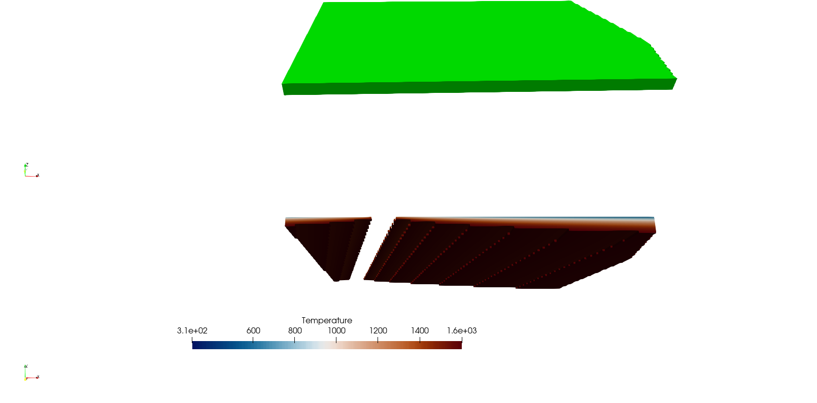
Geometry of the oceanic plate defined with half space cooling temperature model.#
Grains#
Grains model in GWB is used to simulate crystal preferred orientation or lattice preferred orientation (CPO/LPO) within each composition. These are invoked within a "grains models" list in an oceanic plate definition and applied over the specified depth or spatial domain. The depth in meters to which the composition of this feature is present can be given as min depth and max depth. A list with the integer labels of the composition defined using compositions and the labels in rotation matrices. Euler angles z-x-z defines the angles of the grains for each compositions and grain sizes define the size of all of the grains in each composition. If set to <0, the size will be set so that the total is equal to 1. The orientation operation is an option to set whether the value should replace any value previously defined at this location or add the value to the previously define value (add, not implemented). Replacing implies that all values not explicitly defined are set to zero.
Uniform model: This model applies a constant grain across the specified domain.
Random Uniform Distribution: This model applies random uniform distribution [0,1] to each grain using the Graphic Gems III method, which are then set to the rotation matrices. The deflection for the rotation about the pole is constant.
Random Uniform Distribution Deflected: Similar to the previous model but with an additional option of setting the
deflectionsparameter, which lies between [0,1].
Velocity#
The composition of the model can be initiated with a velocity defined in this model. The depth in meters at which this feature must be present can be given as min depth and max depth. The following velocity models are supported:
Uniform raw model: A constant
velocityin meter per year is applied. The coordinates must be in cartesian coordinate system.Euler pole model: To obtain a angular velocity this model can be used. The
euler poleandangular velocityparameters define the (longitude, latitude) in degree and rotational velocity of the Euler pole in degree/Myr respectively. Spherical coordinates is generally preferred but internally support to convert cartesian coordinates to spherical is provided. In that case, a normalization is applied to the coordinates before computing the angular velocity.
Topography#
Topography models enable adding topographical features to the original composition. These serve the need when you want a predefined topography for your geodynamic or landscape evolution model runs. The depth in meters to which the composition of this feature is present can be given as min depth and max depth. The following topography models are supported:
Uniform: A user-defined constant
topographyin meters is added to the composition.Depth surface: The
topographyin meters is added on the coordinates where the depth of surface is defined.