Mid-ocean ridge with a transform fault#
The goal of this tutorial is to learn how to set up a model of a mid-ocean ridge with a transform fault, reproducing the setup of Behn et al., 2007: Thermal structure of oceanic transform faults. In addition, this tutorial shows how the created Geodynamic World Builder file can be used as initial condition for the geodynamic modeling code ASPECT. The corresponding cookbook for setting up the ASPECT model can be found here.
The first step is to prescribe some global parameters for the GWB. This is important because we use the half-space cooling model to compute the temperature distribution within the oceanic plates, and this model uses the thermal diffusivity. In addition, the GWB needs to know what the adiabatic gradient is to compute the correct temperature, and we need to specify the surface and mantle temperature to be consistent with the study we want to reproduce.
Specifically, we here want to set the surface temperature to 0 degrees Celsius (273.25 K) and the potential mantle temperature to 1300 degrees Celsius (1573.25 K) as in Behn et al., 2007. Since that study does not include adiabatic heating, we need to set the thermal expansion coefficient to zero. To reproduce the temperature profile shown in Figure 2 in Behn et al. (2007), we set the thermal diffusivity to 1.06060606e-6 m2/s (which corresponds to a thermal conductivity of 3.5 W/m/K assuming that the density is 3300 kg/m3 and the specific keat is 1000 J/kg/K). Note that we need to make sure that these properties are consistent between the Geodynamic World Builder input file and the input file of the geodynamic modeling code that we are using this file as an initial condition for, in this case ASPECT.
3  "surface temperature":273.15,
4  "potential mantle temperature":1573.15,
5  "thermal expansion coefficient":0,
6  "thermal diffusivity":1.06060606e-6,
 1{
 2  "version":"1.2",
 3  "surface temperature":273.15,
 4  "potential mantle temperature":1573.15,
 5  "thermal expansion coefficient":0,
 6  "thermal diffusivity":1.06060606e-6,
 7  "features":
 8  [
 9    {
10      "model":"oceanic plate",
11      "name":"oceanic plate A",
12      "coordinates":[[-1e3,-1e3],[251e3,-1e3],[251e3,101e3],[-1e3,101e3]],
13      "temperature models":
14      [
15        {
16          "model":"half space model",
17          "max depth":100e3,
18          "spreading velocity":0.03,
19          "top temperature":273.15,
20          "ridge coordinates":[[[200e3,-1e3],[200e3,50e3]],[[50e3,50e3],[50e3,101e3]]]
21        }
22      ]
23    }
24  ]
25}
As the next step, we prescribe the geometry and other properties of the oceanic plate. To do this, we create a feature of type oceanic plate, which we call oceanic plate A. We specify the coordinates where this plate should be present in the model. In this case, we want the whole model domain to be within the plate, so we choose coordinates that span the whole model domain, starting with the x=0 and y=0 corner and then going counterclockwise (increasing the x coordinate first) to all other corners at the surface.
In addition to the location, we also need to specify the temperature distribution within the plate.
To be able to do this, we need to provide the following information to the model: model, ridge coordinates, spreading velocity and max depth. Please see /features/items/oneOf/4/temperature models/items/oneOf/2 for more info.
Here, we use a half-space cooling model (using the material properties we have already prescribed globally) as the temperature model. The full spreading rate is 6 cm/yr, so we need to prescribe a spreading velocity of 0.03 m/yr for the oceanic plate feature since the spreading velocity describes how fast the plate moves away from the ridge.
We also set the top temperature to 0 degrees Celsius (273.25 K), determining the temperature we use as the surface temperature in the half-space cooling model. Finally, we need to specify the coordinates of the mid-ocean ridge segments. Both segments are parallel to the y-axis, with the first segment being located at x=200 km, going from y=-1 km to y=50 km, and the second located at x=50 km going from y=50 km to y=101 km.
 7  "features":
 8  [
 9    {
10      "model":"oceanic plate",
11      "name":"oceanic plate A",
12      "coordinates":[[-1e3,-1e3],[251e3,-1e3],[251e3,101e3],[-1e3,101e3]],
13      "temperature models":
14      [
15        {
16          "model":"half space model",
17          "max depth":100e3,
18          "spreading velocity":0.03,
19          "top temperature":273.15,
20          "ridge coordinates":[[[200e3,-1e3],[200e3,50e3]],[[50e3,50e3],[50e3,101e3]]]
21        }
22      ]
23    }
24  ]
 1{
 2  "version":"1.2",
 3  "surface temperature":273.15,
 4  "potential mantle temperature":1573.15,
 5  "thermal expansion coefficient":0,
 6  "thermal diffusivity":1.06060606e-6,
 7  "features":
 8  [
 9    {
10      "model":"oceanic plate",
11      "name":"oceanic plate A",
12      "coordinates":[[-1e3,-1e3],[251e3,-1e3],[251e3,101e3],[-1e3,101e3]],
13      "temperature models":
14      [
15        {
16          "model":"half space model",
17          "max depth":100e3,
18          "spreading velocity":0.03,
19          "top temperature":273.15,
20          "ridge coordinates":[[[200e3,-1e3],[200e3,50e3]],[[50e3,50e3],[50e3,101e3]]]
21        }
22      ]
23    }
24  ]
25}
The figures below show the resulting thermal structure of the model.
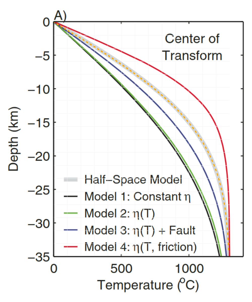
Temperature profile at the center of the transform fault. Output from the Geodynamic World Builder (orange dashed line) plotted on top of Figure 2a of Behn et al., 2007, showing good agreement with the half-space cooling model from that study.#
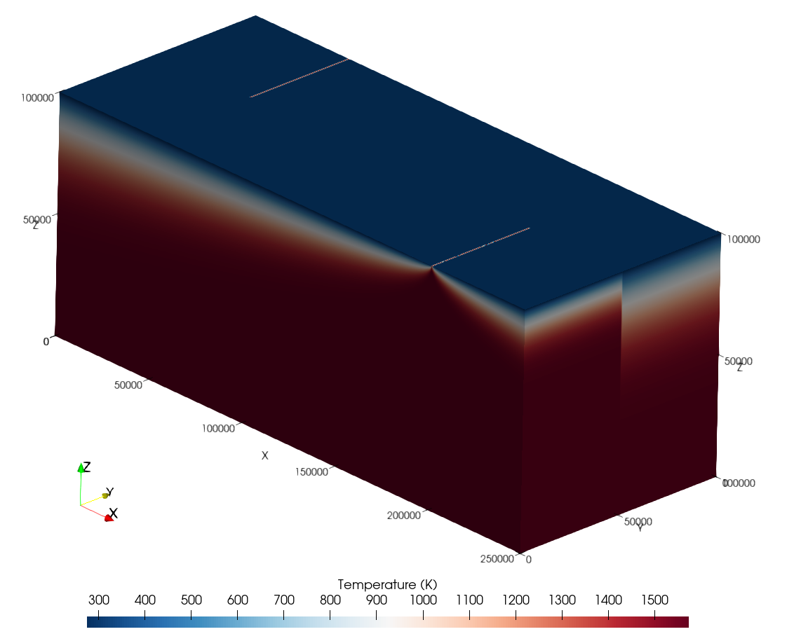
Transform fault geometry and temperature distribution.#