Subducting plate oceanic part

Now that we have made the overriding (Caribbean) plate, it is time to add the oceanic part of the subducting plate (the Atlantic). To do this, we just need to add another object to the feature list. For this plate we will assume the oceanic lithosphere is really old, and the temperature gradient in the lithosphere is therefore linear between a top temperature of 293.15K and the adiabatic temperature at the max depth of the plate. Luckily for us, this is the default in the world builder, so we will only need to provide the model (linear) and the max depth, which we will set to 100km.

For the composition, we are going to do something a bit more special. A common thing you will probably want to do with compositional fields is have multiple layers of them within a feature. This is very easy to do in the GWB. If you remember from the last section, both the temperature models and compositional models are a list of objects. Making layers is thus as easy as adding multiple compositional models with each their own min depth and max depth.

Note

If you provide a min depth or max depth outside the min and max depth range of the feature, it will be cut off by the feature min and max depth range.

Important lines

    },
    {
      "model":"oceanic plate", "name":"Subducting Oceanic plate", "max depth":100e3, 
      "coordinates":[[2000e3,0],[2000e3,1000e3],[1500e3,1000e3],[1600e3,350e3],[1500e3,0]],
      "temperature models":[{"model":"linear", "max depth":100e3}],
       "composition models":[{"model":"uniform", "compositions":[3], "max depth":50e3},
                             {"model":"uniform", "compositions":[1], "min depth":50e3}]
    }

BST_07_subducting_plate_oceanic_part.wb

BST_07_subducting_plate_oceanic_part.grid

Paraview v2 state file

Full file

{
  "version": "1.0",
  "coordinate system":{"model":"cartesian"},
  "features":
  [
    {
       "model":"oceanic plate", "name":"Overriding Plate", "max depth":100e3, 
       "coordinates":[[0,0],[0,1000e3],[1500e3,1000e3],[1600e3,350e3],[1500e3,0]],
       "temperature models":
         [
           {"model":"half space model", "max depth":100e3, "spreading velocity":0.04, 
            "ridge coordinates":[[[400e3,-1],[-100e3,2000e3]]]}
         ],
       "composition models":
         [
           {"model":"uniform", "compositions":[0], "max depth":50e3}
         ]
    },
    {
      "model":"oceanic plate", "name":"Subducting Oceanic plate", "max depth":100e3, 
      "coordinates":[[2000e3,0],[2000e3,1000e3],[1500e3,1000e3],[1600e3,350e3],[1500e3,0]],
      "temperature models":[{"model":"linear", "max depth":100e3}],
       "composition models":[{"model":"uniform", "compositions":[3], "max depth":50e3},
                             {"model":"uniform", "compositions":[1], "min depth":50e3}]
    }
  ]
}

BST_07_subducting_plate_oceanic_part.wb

BST_07_subducting_plate_oceanic_part.grid

Paraview v2 state file

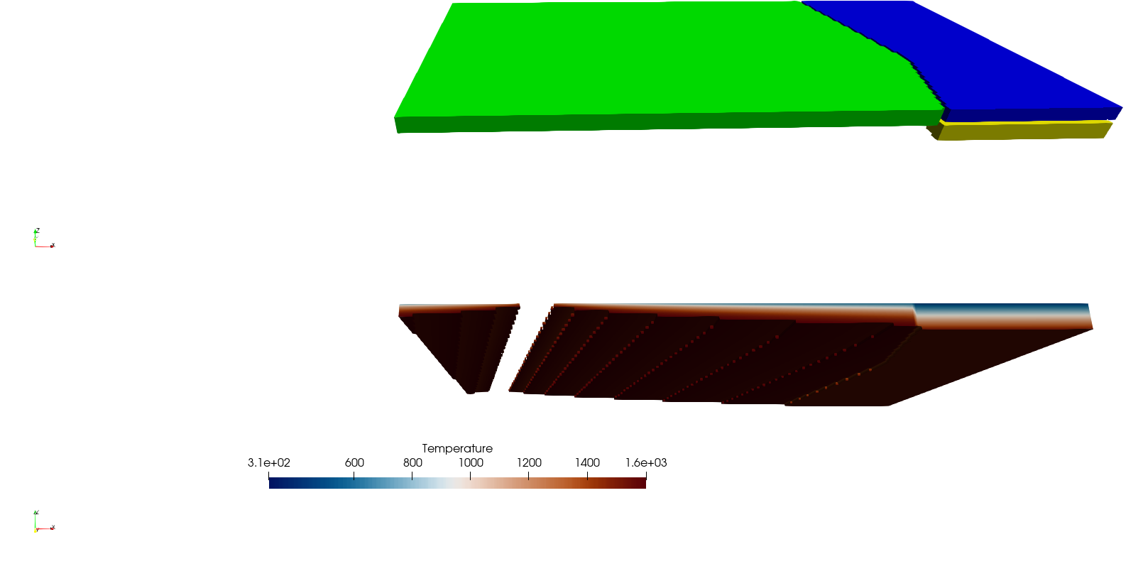
Basic Starter Tutorial section 7. The top part of the figure shows where the composition as been assigned as an object. Currently is shows composition 0 as green, composition 1 as yellow and composition 3 as blue. The bottom part shows the temperature as seen slightly from below where only temperatures between 300K and 1600K are shown. Both the oceanic plate with the ridge and the oceanic plate with a linear temperature profile are visible.